Rebase curve upgrade proposal

Summary

Change the rebase factor function from a linear curve to an S-shaped curve.

Abstract

The proposal is to deploy a new contract that updates the current supply policy’s linear rebase function with a Sigmoid function.

Motivation

The original Ampleforth linear rebase function was intended to make minimal assumptions about how price reacts to expansion and contraction–i.e. expansion would slow price increases by translating them into supply increases and contraction would slow price decreases by translating them into supply decreases. Hence the main purpose of the function is to point supply change in the right direction without trying to predict the exact magnitude of supply change needed for the fastest convergence to the price target.

At this point in time there is history to analyze and use to improve the rebase curve accordingly. e.g, we can see that extreme market scenarios can have outsized effects on AMPL supply, which then require prolonged supply corrections. The linear curve is very limited on how it can be configured and an S-shaped curve can allow for more sophisticated tuning of the rebase function.

The advantages of an Sigmoid curve:

  • Can be configured to have different slopes at different points of the curve.

  • It has bounds (asymptotes)

    • That makes AMPL supply changes relatively more predictable beyond the current day
    • Limits the potential effect from a bad oracle price. This makes AMPL more resilient to errors and attacks and also increases the feasibility of further oracle decentralization efforts.

Specification

The smart contract upgrade replaces the current linear rebasing function with a sigmoid curve that caps supply changes at its asymptotes

Rebase factor of 1.0 means no rebase.
Normalized price = VWAP price / Target price

The proposed curve above is generated by the sigmoid function:

F(x) : fraction of supply added or removed (supply change %)

x : normalized price deviation

NOTE: x in the formula above is normalized price deviation and F(x) is the fraction of change while the diagram for better visual representation shows the normalized price on the x-axis and the supply multiplier factor on the y-axis.

It has shaping parameters that determine: lower asymptote, upper asymptote, and the steepness of the curve (ie: growth rate).

l = lower asymptote
u = upper asymptote
g = growth rate

Technical Specification

This update creates no changes to external APIs. Clients, including exchanges that listen to AMPL’s rebase events, will still receive the absolute supply change integer as before. However, note that any external application that calculates the supply change independently will need to update their calculation logic.

Parameter Values

The parameters are chosen to be very similar to the current curve in the normalized price range of ($0.5 to $1.5) and caps the changes to 10% on the expansion side, and that caps the contraction side at -7.78%

The proposed values are:

l (Lower) = -0.1
u (Upper) = 0.1
g (Growth) = 3

Test Cases

Existing unit tests will be updated with the correct calculation results to maintain test coverage.

Conclusions

The Ampleforth protocol will maintain the same nature to change supply to match demand. And the new curve would allow further improvements by changing the sigmoid parameters, which is independent from this AIP.

4 Likes

Reposting the question I asked about this topic during one of the Amphitheater sessions. I think it’s good to have a written answer to this question:

Wouldn’t capping the max rebase with AIP-5 increase price volatility dramatically?
Basically all the excess buying (that go beyond $2) cannot be dampened with rebases anymore so it will translate into higher price fluctuations instead.

If for example there was massive demand for AMPL pushing the marketcap 10x to 3billion, since rebases are capped, we might see the higher marketcap now being reflected in price instead, like 3$ 4$ AMPL?

That being said, I’m in favour of this proposal
(edit: as long as the curve is steeper than before)

Rebases are going to be stronger for prices where AMPL has spent the most time in the past, allowing for quicker supply adjustments.

It’s also going to avoid the extreme scenarios where very high positive rebases would overshoot the optimal supply for the market condition and then be followed by prolonged correction in supply that would last unnecessary long.

Max rebase to me is counter intuitive to the dampening procedure of the protocol. Also the “predictability” in rebase that OP touts only applies in one direction and is sort of a red herring to the purpose of the protocol which is elasticity.
Cubic rebase function fixed these concerns

I don’t really see the advantages of a rebase cap. It adds complexity to something which was born simply and easy to follow. In addition, by limiting the rebase it will even take longer for supply to get back to its equilibrium. Interesting proposal but at this point I think it’s better to keep concepts simple and straightforward, otherwise we will never gain general adoption.

I just saw the pictures.

The sigmoid curve graph that you provided looks different than the one that was shown here: AIP-5: Sigmoid Rebase Function

Is it different now @Naguib ? I wouldn’t support a max rebase cap without the steeper curves in the middle.

Going to start off by saying this is pretty exciting, a lot of work and time has probably gone into this. I think supply policy is a very delicate topic - being that it’s the core of Ampl’s identity.

I think in general I am in favour of at least experimenting with a sigmoid curve to see how it affects Ampl’s ability to return to target. I think there’s several more things that we should outline in this discussion before we proceed though:

1. How long do we plan to try this for before doing a check-in? Are there any conditions that will require us to emergency revert, or is it a play-it-by-ear situation?

2. What metrics will be using for judging? I am inclined to think that since the motivation is to mitigate the effects of extreme market scenarios that results prolonged supply corrections, that the only metrics we should look at are:

  • time to return to target price, and
  • time spent at target price range

3. What is our justification/strategy for the parameters that we pick?
I am inclined to agree with @Togenkyo here that a larger/steeper supply change is what would help with Ampl returning to it’s target price more quickly. Ganesh proposed some alternatives that also follow this approach.

On a side note I am personally curious why we think “predictability” of Ampl’s supply out into the future is what will help it return to target faster? I think intuitively that it seems to make sense (i.e. less predictability =>, more speculation/gaming) - but would be good to have the logic clearly laid out for anyone who may not be following.

1 Like

In an extended period of price above target and positive rebase, there are multiple actors among them are:

  1. Selling at increased market cap due to both price and supply increasing.
  2. Buying based on expectation that market cap increase will result in growth of holders.

The behavior of actor 2 has been seen to drive the market cap up beyond the supportable market cap and hence results in a sudden and steep price decrease to or below target price. Having a slower supply expansion can cool that effect which would in return cool down the price drop after a period of expansion.

Rebases are going to be stronger for prices where AMPL has spent the most time in the past, allowing for quicker supply adjustments.

That is not the case with this version of the proposal this one is matching the current linear curve for most of the price range.

Yes this proposal is introducing a sigmoid curve with a minimal change from the current linear curve. And in later proposal configure parameters to achieve better performance. As opposed to bundling the changes in one go.

I ran a simulation of AMPL’s historical data with the sigmoid function applied instead of the linear formula. Thanks to AMPLtools for the handy data, and I also used Coingecko to fill in missing values. I’ll upload my calculation spreadsheet to the governance channel on Discord so others can verify.

This simulation makes one critical assumption, and that is unchanged demand from historical demand. In other words, for both the linear rebases and sigmoid rebases the price*supply (market cap) is unchanged. Given an unchanging demand, I’ve simulated prices and supplies (circulating and total) for all dates.


Prices seem to track very closely except for the massive expansion in July 2020, where the sigmoid rebases result in much greater price divergence from target, almost reaching $7.


A similar but inverted picture appears with circulating supply, where sigmoid supply volatility is temporarily dampened during the big July 2020 expansion but otherwise matches the linear supply volatility closely.


Total supply shows a similar pattern.


You can see here the “capping” of rebases by the sigmoid function at a max of 10%.

Overall, I think this demonstrates that the sigmoid rebases are functionally identical to linear rebases except for the rare scenarios of exceptionally high or low demand. When demand changes rapidly, the sigmoid rebases appear to result in greater price volatility and dampened supply volatility. It’s up to the AMPL community whether they value price stability over supply volatility, and choose the corresponding rebase pattern. Personally, I think that price stability is more desirable and so I oppose the switch to the sigmoid rebase but on the whole I think it will have little effect on AMPL in the long term.

8 Likes

@ducc
Great work running the simulation!

Curious how for some dates the sigmoid curve is higher for both price and supply if the assumption is that market cap is equivalent.

This simulation makes one critical assumption, and that is unchanged demand from historical demand. In other words, for both the linear rebases and sigmoid rebases the price*supply (market cap) is unchanged.

Given that on a given day, the trajectory of previous rebases and expected rebase has shown to affect demand. Check my reply above to @Togenkyo mentioning two behaviors of the possible market actors to supply expansion. Such a neat simulation is not useful to predict price response to a different rebase function. It does show, though, that this proposal is equivalent to the current curve for most of the historically relevant price range.

@Zezima @Vihtori

Max rebase to me is counter intuitive to the dampening procedure of the protocol.

limiting the rebase it will even take longer for supply to get back to its equilibrium.

It may take more days but it is still significant enough to catch up with demand. While giving time to distinguish between short bursts of high demand vs sustainable increases in demand.

“predictability” in rebase that OP touts only applies in one direction and is sort of a red herring to the purpose of the protocol which is elasticity.

I think you are referring to different predictability than what’s referred to in the proposal. The predictability referred to in the proposal is that in one rebase action there would be a limit to the supply change. This increases usability of AMPL with other applications and protocols. e.g., Lending having bounds for rebase reduces liquidation risk and makes the risk more quantifiable. Improving AMPL’s performance as a collateral.

@G-Yes95

  1. How long do we plan to try this for before doing a check-in? Are there any conditions that will require us to emergency revert, or is it a play-it-by-ear situation?

Given the minimalism of this change from the current curve that shouldn’t be a concern.

  1. What metrics will be using for judging?

Factors to monitor (Without getting into their formal specification):

  • Fluctuations of market caps at the end of expansion and contraction periods, as this measures if contraction and expansion are overshooting the market cap/supply that matches the demand.
  • Time to get back to the target once diverged.
  • Time around target
  1. What is our justification/strategy for the parameters that we pick?

For this proposal the parameters are set in a way to have minimal change to the current linear function.
In broad terms for potential future configuration proposals the goal is reducing price and supply volatility.

1 Like

So having thought about this more, I think this ultimately comes down to where we expect demand is coming from (and where expect it to come from in the future) during expansion periods. If demand is expected to remain constant for some sort of utility, then I think more price volatility is expected as ducc suggested. If demand is primarily from short-term-speculative activity, then it’s possible that capping the rebase prevents the demand from ever increasing that high to begin with. I.e. if you’re a short-term-speculator and you know that Ampl rebases the ~same at $1.5 vs at $2, would you still buy it for $2? For $4?

I think that demand (thus far) during positive rebase is primarily from speculators. Below is some data that suggests that is the case:

Back during Defi Summer is when geysers were launched, which was arguably the first “utility”. We can see that at Point C, there was a OOM increase in new addresses with coincided with the geyser launch. This was propogated to the red curve (Cruisers 1-12M) roughly 1 month from the peak of Ampl price. This was then propogated to the blue curve (Hodlers 12M+) roughly 1 year at Point B(agholders).

The interesting thing is that since Defi Summer, the grey curve has been fluctuating, but you don’t see an equally proportional propogation into the red curve. If there was truly utility driven demand, I imagine we would’ve seen something like this instead:

There’s also transaction data. There is a considerable shortening of average time between transactions right before and during positive rebase phases. Something similar can be seen with transaction volume and transaction count.

It’s important to note that any one of these indicators by themselves likely aren’t conclusive evidence of anything, but combined with the address by time held data above - I think it’s largely reflective of price activity primarily being driven by short-term-speculators, aside from a couple exceptions.

Having said that, if we consider that Ampl is now in the utility era, that will likely bring speculators with it as utilities continue launching. However, the demand from short-term-speculators should get drained out before Ampl Price strays a certain amount from it’s target.

Ultimately I find myself in agreement to some degree with all the different opinions presented thus far:

  • I agree with Naguib’s take that capping the rebase factor will mitigate the effect of short-term-speculators on the price, making the price a more reliable measure of sustained demand
  • I agree with Ducc’s take that this will lead to short term price volatility in the short term with large-sudden-demand changes, especially with utilities launching
  • I agree with Tog’s take that a steeper slope near the price target is worth exploring (in the long run)

Ultimately, i think that with the parameters proposed today, it’ll give us a quick indication (while taking on less risk) of whether this deters “run-away-speculative activity”. If parameters will be adjusted in the future to account for the utility driven demand, then I am for implementing this.

Data source: intotheblocks.com

8 Likes

I appreciate the data gathering and simulation to try and predict what might happen if we switch rebase functions. I do fear that because price changes affect how demand is distributed, that these models are limited on what they can predict, however, and we have had a very critical assumption leak into our supply policy which is affecting our price and supply data. For the record I favor this proposal and I’m going to take a different approach and arguing for this change. There are two main points to this argument, a mathematical symmetry argument, and a psychological argument.

Linear function was used to make no assumptions about how supply changes should change, but in fact there was a hidden assumption. Now a linear function is the simplest function and easiest to understand and looking at a graph, it looks symmetrical, but for this use case it is not. This is because while price can go above 100% price target, the price can never go below 100% of the price target. This creates a lopsided supply adjustment curve, and during periods of supply shocks, whether increasing or decreasing, the supply changes are lopsided towards growth.

Lets take an example, price of AMPL goes to +50% price target, that represents a 50% market cap gain, and results in a 5% first daily rebase. The flips side is -50%, and that results in a 50% market cap loss, and the supply contracts 5%. This seems symmetrical and one might think time in growth and decay on average should be about the same. Now what if we go +100% price target, to about 2$? This means that the supply changes 10%, trying to quickly respond to the change in demand. Now what if we need to correct back down to the previous market cap? Well, the price cant go to 0 for a 10% negative rebase, what gives?

There’s something deeper here, and that if the supply increases 10%, that corresponds to a 100% increase in market cap at the price target, and that means if we want to correct back down to previous market cap, we only need to reduce the market cap by 50%. Therefore it would make more mathematical sense to have this match, the rate of change of supply should be proportionally the same to what it would take to return the previous market cap after expansion. So if the supply increases 50%, the rate of change of supply expansion should match the rate of supply contraction if the market cap decreases 33%. NOTE this is exactly how fixed supply market caps change! 50% increase in price requires a 33% decrease to return to previous market cap. The difference with AMPL is we have rate of change of supply to add to the equation, but that rate of change should be proportionally similar to how the marketcap changes in standard tokens if we really do not want to make assumptions about how the supply should change. Some math whiz please formulate this for me :slight_smile:

If we agree on the above the things left to debate are what should the magnitude of the change be as we go away from the price target (either up or down), but I think it is critical that we balance the rate of change so movements up and down are symmetrical.

Now we understand why most of the time the community has felt negative rebases. This is because our expansions are relatively faster then are contractions!!. All it takes is one large outsized supply expansion to create a much longer period of supply contraction! Now that AMPL is starting to mature more and we are getting more utility, I want us to fix this as a community because as a true AMPL believer I want long term sustainable growth of the community. And now on to the psychological aspect of the argument.

The lopsided nature of supply expansions and contractions has a negative effect on the community. This supply curve, and history shows, that a lot of time is spent in negative rebase territory. Lowering value a strong psychological effect on holders, because more times then not when you buy in, you spend most of your time losing money. This makes it harder to grow the community in general, and lowers morale because most of the time people are getting burned, and it requires deep belief in the fundamentals of the project to stick with it. I want as many people as possible to get into AMPL, but I dont want them fearing forever bear markets, as most of the time we are in because of the current rebase function design.

Think about how people who got burned by banks going under hoard cash or gold, and will never go back. There are probably tons of people who could have been potential community members but couldn’t stick through this massive bear cycle in AMPL’s history. The less time we spend in negative rebase territory, the easier I believe it will be to sustain organic growth in the community.

So therefore I am in favor of the sigmoid function tuned to match something similar to the supply policy I listed above, if I have time I can try to figure it out mathematically but I know we have a lot of smart people in here that can also figure it out. Lets finally make AMPL symmetrical. Cheers

8 Likes

I don’t know where you’re seeing that. I posted the spreadsheet in the discord governance channel if you’d like to check the raw values for yourself. Price*circulating supply is identical for both rebase conditions for every day.

Do you have some evidence for this? I’d be very interested to see.

As far as I understand, with the newly proposed parameters the sigmoid curve only introduce an asymptotic property for price ranges outside of [0.92, 1.08] with 1 being the current CPI value. Inside the “normal” price range the new curve will be nearly identical to the current linear one.

I’m in favor of the asymptotic properties for the following two reasons:

  1. Supply adjustments will be less prone to extreme price jumps
  2. The oracle infrastructure will be more resilient to faulty values

My understanding of Amples mantra, “moving price volatility to supply volatility”, is that the supply should, whenever possible, be only adjusted for sustainable changes in demand. I think short term price fluctuations don’t need to be translated into supply as this supply adjustment would soon need to be bounced back anyway. @ducc’s visualizations above seem to support this point.

Some more context for community members joining the discussion at some point in the future:

3 Likes

Okay I changed my mind, I’m not in favor of sigmoid, I’m in favor of | log(x) |, see my post here Symmetric Rebase Upgrade Proposal

Another idea I think that should be explored… can we combine the symmetric properties of the natural logarithm with the stabilizing shape and flexibility of a sigmoid?

Okay I think I figured something out. If we compose the natural log function in the sigmoid function we get the symmetric property I talked about in Symmetric Rebase Upgrade Proposal, we can “scale” x to balance out expansion and contraction. I modified the code in @aalavandhan1894 notebook to illustrate this:
Google Colab

I think with this we may get the best of both worlds… no longer skewing rebases to faster expansions followed by slower contractions, but also giving us the tools to elegantly cap each side and tune the shape

Edit: Cross-posting from the Symmetric Rebase post, @Togenkyo made a nice visualization of all the rebase functions we’ve been evaluating. Symmetric Rebase Upgrade Proposal - #8 by Togenkyo

I’d like to highlight how the Sigmoid Function behaves with changing parameters:

u = 0.1, l = -0.1, g = 3

u = 0.11, l = -0.11, g = 4

The Sigmoid Function opens up the possibilty to adjust the rebase curve for prices where AMPL is spending the most time at, while also adding a rebase cap for extreme scenarios.

1 Like

PREFACE

Hey all,

There’s been a lot of good discussion for this topic, and I’ve seen excellent points brought up from just about everyone. I think we should collectively spend a lot of time trying to understand everyone’s concerns, because I believe all opinions are bringing some good points to the table. The free market is the greatest computation engine to ever exist. The aggregated effects of our purchasing decisions ultimately reflect itself in the market data. In this piece, I will explain how we can implement a solution that combines the best of all the opinions I’ve seen so far.

ABSTRACT

The most optimal solution is a combination of a sigmoid and cubic function. The protocol would need to apply the rebase according to minimal history about it’s state. This is analagous to hysteresis in the natural world => making AMPL a sort of digital steel counterpart to BTC as the digital gold.

PROBLEM STATEMENT

We should make it crystal clear that the purpose of this protocol is to be a unit of account. That has been implemented with our beloved token that returns to it’s price target → without any collateral or lender of last resort. We have seen that Ampl eventually reaches it’s price target, which is a can be thought of as a reflection of the economic theory of supply and demand. However it is not enough to simply reach price target eventually, as the maximum benefit is achieved when Ampl is doing the following:

• As close to it's target price as possible 
• At it's target price for as *long* as possible 

The goal of this protocol is not any of the following:

• Have a constant supply 
• Have an exponentially growing supply 
• Have a constant market cap 
• Have an always up market cap 

The things above will be a result of Ampl staying at it’s price target. They are measures of the usefulness of the protocol. By Goodhart’s Law , when the measurements become targets, they cease to be good measures.

Having said that, if we want to improve AMPL’s price stability, we must look at why price has been following the trend it has, and the supply charts may be helpful for visualizing that. We must first come to alignment on the root cause if we are to come up with an appropriate solution.

OBSERVATIONS

The primary motivation for this endeavor has been stated as being that Ampl’s price spends a relatively short amount of time above it’s target price, but spends long periods of time below it’s market cap. If we want to understand this then we must understand the four things below:

• Why does Ampl's price rise rapidly when it is in expansion (the RIP) 
• Why does Ampl's price fall quickly when after it has reached the peak of expansion (the FLIP)
• Why does Ampl's price fall quickly when it is near target after expansion (the DIP)
• Why does Ampl's price rise slowly back to target (the TRIP)

image

I’ve shown in my earlier post the data that strongly suggests price activity mainly being driven by short-term-speculation and fast-moving-traders. To help understanding them, we need only apply some staged Game Theory to understand how they think. If we believe our hypothesis is correct, we can revisit the historical data to see if it matches our analysis. We can use a 2x2 matrix where there is Player A and Player B. Their options are to buy & sell.

• If both players prefer to buy, price rises. 
• If one player is buying and one is selling, price is unchanged. 
• If both players sell, price falls. 

Extending that, Ampl is designed so that:

• when both players buy, we have expansion 
• when both players sell, we enter contraction 
• When only one player buys, and the other sells, supply is neutral. 

Part A - THE RIP

Currently the protocol is designed such that if both players buy when initially at neutral price, then we will enter expansion. This actually benefits both players. If both players sell, then we would contract which punishes both players. If one is buying and one selling, then there is no reward. This is a zero-sum game, which is why Ampl eventually always returns to its target. Given that this is played in multiple turns, the sum of all plays for Player A and Player B = 0. It’s also symmetric in that it doesn’t matter if Player A uses Player B’s strategy.

At any given instant where price is neutral, there is a Strictly Dominating strategy. Regardless of what the other player is doing, it’s in the benefit for Player A & Player B to buy. This is what causes the price to rise so rapidly out of Price Target Zone.

Part B - THE FLIP

After Ampl enters expansion, the players switch to playing a classic Stag Hunt game. Applied to our protocol, it would look something like this:

In this game, there isn’t a strictly dominating strategy. This game has a Nash Equilibrium, where each player is incentivized to match what the other player is doing. I.e. if Player A is buying, Player B will also buy. However if Player A decides to sell, then Player B also decides to sell. This is a pure strategy.

And this lines up perfectly with we observe in the charts! Given that we just entered expansion with a RIP, Player A/ Player B assume that the other is buying and matches them. The price continues rising… until someone sells a large enough volume to kick the game out of Nash Equilibrium and towards the new Nash Equilibrium of selling.

PART C - THE DIP

If Player A and Player B both sell, it will cause prices to fall. However, we can observe that Player A and Player B have a tendency to over-shoot. As a result, price will actually quickly fall below price target, causing Ampl to contraction. During contraction, it is still a Stag Hunt game, for which the Nash equilibrium is staying in contraction. This is why Ampl enters contraction so soon after reaching the top of it’s supply curves.

PART D - THE TRIP (back up)

However we’ve observed that Ampl’s price doesn’t continue dropping indefinitely. Moreover, it takes a long time to return to target after reaching expansion. There are a few reasons for this:

1) Humans are biased with loss aversion. Losing $100 feels way worse than winning $100. As a result, the force/disturbance required to move the Stag Hunt game out of equilibrium is much higher than the disturbance required to kick it out of Nash equilibrium during expansion. 
2) Despite being in contraction, there are a small amount of buyers speculating on expansion soon :tm: These buyers are very slow.
3) The remaining volume every day during contraction can be attributed to the liquidity pools. When Ampl contracts (all else being equal), the paired tokens will be sold for Ampl in order to keep the pool weightings the same. Investors who have decided to stake their Ampl in liquidity pools have been keeping the buy pressure afloat. As long as those investors are not withdrawing their liquidity, these pools help act as a slow but nudging force. This is very observable in particular when the wider market is trading sideways. Ampl appears to nudge higher slowly, with some small spikes of considerable volume. 

When the price eventually reaches target price, the cycle repeats.

Summary so far:

If we apply the theory that there’s a cost to switching between games, then it’s ultimately more efficient to just continue playing the stag hunt game. Yes we always reach price target (opposite moves), but that’s a short detour to the new Nash equilibrium in expansion or contraction. And due to loss aversion, it’s easier for a disturbance to kick the system out of expansion than it is to kick it out of contraction.

Imo this model lines up perfectly with the market data - which is showing us that for the current set up, it’s literally more efficient to spend as little time in neutral range as possible.

Proposed Solutions so Far:

There have been a number of proposed solutions:

@Naguib
@Zezima
@Togenkyo
@kbambridge

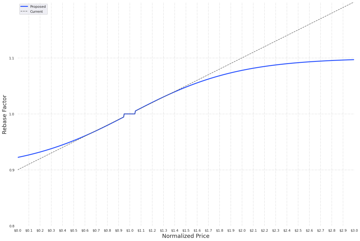
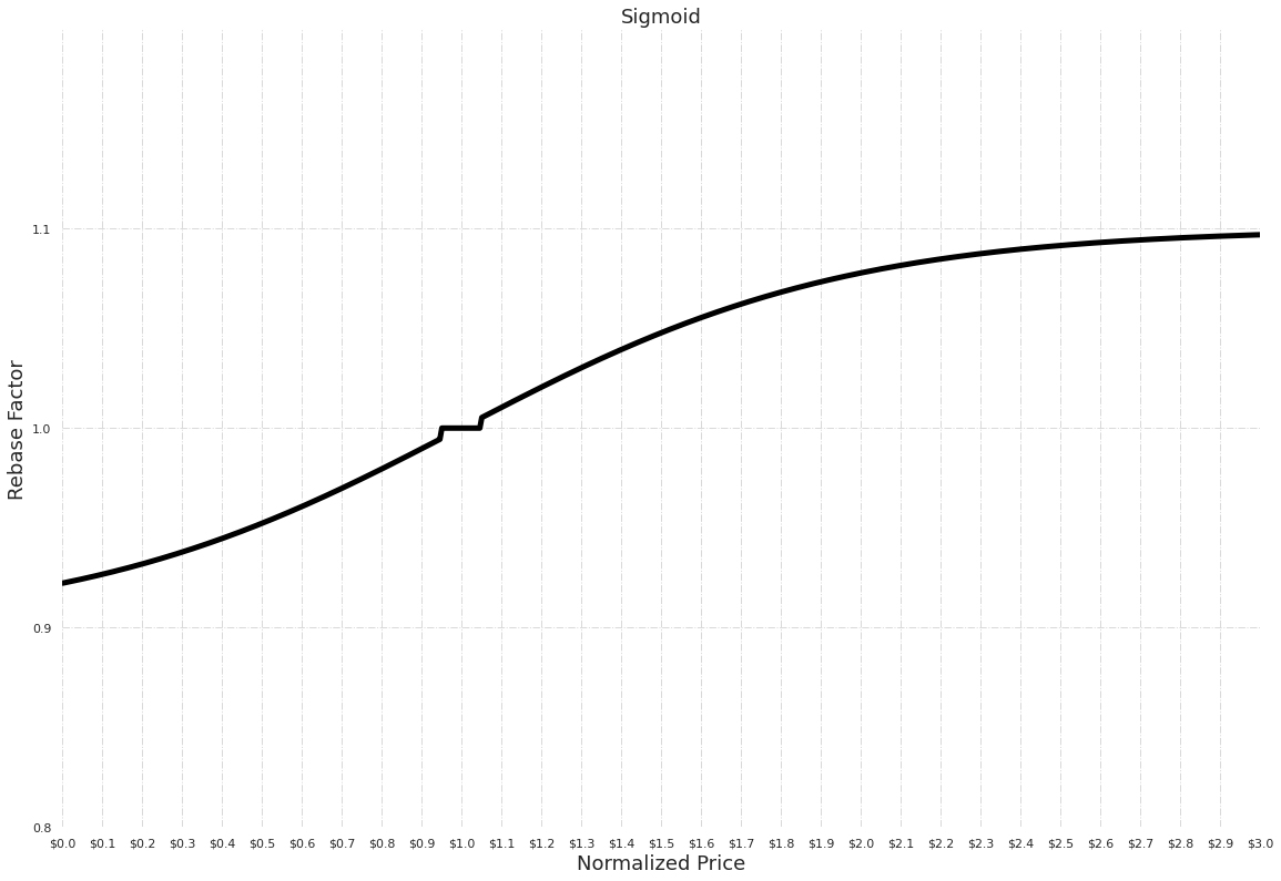
1) Sigmoid function -> cap the positive rebase to disincentivize speculators from driving the price up 
2) Cubic function-> the idea behind this is to incentivize heavy selling when there is large expansion by the laws of supply and demand 
3) Steep slope-> this attempts to further the benefits of sigmoid by forcing the rate of increase of rebase to decrease before reaching high levels 
4) Logarithmic input  -> this attempts to symmetrize the rebase value as a % away from target rather than a raw amount. 

All of these solutions provide benefits, but they’re ultimately incomplete, because they fail to look at what happens over a full cycle of the game.

Below are the criticisms of each:

Sigmoid:
When there is legitimate demand (for a utility perhaps) Player A is revealing their hand by buying. Therefore even the rebase is capped, Nash Equilibrium is still for both players to buy. This feedback loop will continue. Despite rebase growth being throttled, each player’s wallet still grows by a larger amount by buying. Call a spade a spade, it’s still a stag hunt game when away from price neutral target.

Another way of looking at it: Traders ultimately will buy and sell based on their expectation of when others will buy and sell. If you know that supply is not expanding fast enough to accommodate real demand, you will still buy. You might not pay the same price as when it was a Stag Hunt game (since the rebase is capped), but you will still buy.

Side note: This might also explain why some people have commented that sigmoid will do “nothing”.

Cubic Function
This makes the dominant strategy of buying at neutral price even more lucrative by further incentivizing with a higher growth rebase for escaping target price.

Steeper Curves
this attempts to make the throttling of the rebase from Sigmoid happen sooner. Ultimately it’s the same Stag game, and it’s actually worse around neutral price zone for the same reasons that cubic doesn’t work. In some ways, this is the worst by combining both.

Logarithmic Input:
While this solves a problem with respect to how humans evaluate deviation from target, this doesn’t actually address any problem related to the incentives at any point in the cycle of the game.

This is not suggest at all that any of these ideas are useless, however. Far from it.

Strategy for a Wholistic Solution

If we want the best possible solution, we must analyze the game theory as a staged game and design our incentivizes accordingly. Again, coming back to our problem statement, we stated that our goal is to achieve stable price. Therefore we must be targeting an equilibrium where only one player is buying and is one is selling at any given time.

Let us start with the same zero sum game at initial conditions. Since the dominant strategy is buying, we can assume that we start off the same way and enter an expansion phase. After we enter expansion, we can then make the game such that the selling comes the dominant strategy. For that to be the case our expansion matrix would look like this ( forgive muh 3,3 ) :

It’s not enough to disincentivize buying during expansion, we must make it strictly dominant to sell. This is what the sigmoid function fails to do. If we overcorrect and enter contraction, we must again make buying the strictly dominant strategy, which would look something like this:

General Implementation

Traders will sell when their fear of loss is greater than the benefit of the reward.

If we come back to the sigmoid function, there is a cap, which reduces the reward. I.e. disincentivizes buying. This is a good first start. However if we want to make it truly logical to sell, there must be a fear of loss.

One way to do this is to make the rebase drop faster after entering the . Intuitively this makes sense. If rebase can drop much faster than it can rise => then those who sell first, sell best. You’re no longer relying on a disturbance to break a Nash Equilibrium => the restoring force is built into the protocol.

image

In order to adhere to the identity of the protocol to rebase positively above target and negatively target, we would need to make it so that this effect slows down approaching target.

image

On the opposite end, we can apply the same strategy, where the rebase can recover much faster if it went thru heavy contraction. If you look, now, the curves we added look pretty similar to a cubic function. This provides an intuitive explanation for understanding why it has been suggested.

image

Ultimately this means our policy will need to follow a different curve based on it’s history.

Aside

This is comparably observable in the magnetic domain, with Hysteresis loops (where the state of the material depends on its history). When a magnetic field is applied to an iron object: it still remains magnetized even after the field is removed. The flux density can not be eliminated unless a coercive force (i.e a field is applied in the opposite direction) is applied.

image

@evankuo I know you studied MechEng like me, so I hope your Berkeley profs were teaching this instead of cancel culture :stuck_out_tongue:

Jokes aside, this model provides a useful analogy in that if Bitcoin is digital gold, then Ampl is digital Steel. If you haven’t noticed, nearly every man-made structure around you has some form of steel in it. Our whole planet is literally an iron ball at it’s core.

Specific Implementation

The specific implementation would follow something like this:

1) Protocol rebases positively above price target range, negatively below target range, and neutral at target threshold (nothing new here) 
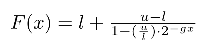
2) If price is slightly above or below target, then it follows the sigmoid function. 
3) If the price into extreme expansion or extreme contraction i.e. above a higher threshold or below low threshold, then a xTremeFlag is set that let's the protocol remember that we are in sustained Demand zone.
4) If TWAP on any given day is less than the previous day, then the rebase applied is according to a cubic function that's fit thru 3 points ( 0, minRebase) (1, 0 rebase) and (lastRebasePrice, lastRebase%)
The function will be of the form y = (ax-b)^3 + c 
5) Once the cubic function mode has been triggered, then that function remains the same. 
6) In order for the flag to clear, the TWAP must be within target price range. 
7) Once cleared, if price reaches new ATHs, then the next time the cubic function mode is triggered is refitted to replace the (lastRebasePrice, lastRebase%)

Checking against our framework

Since the criticism of the existing proposals was that they did not address the whole cycle, it would be hypocritical to not confirm how the wholistic solution holds up according to the game theory.

So if Player A and Player B choose to go into expansion, it’s becomes more strategic to bring it back into to neutral. And if they over-correct and bring it into contraction, then it will be more efficient to bring it back into neutral. However switching between games comes is inefficient on a whole.

In this multi-stage game, the hypothesis is that the market will realize that it most efficient to enter extreme expansion or contraction, only when absolutely necessary. I.e. if there was a new utility that launched, or if there was a security vulnerability (knock on wood).

By virtue of designing the game so that we are around price-neutral target as often as possible, the supply & market-cap shape will purely be reflective of how useful the protocol is - and whether the game is designed well. Take the elevator up and take the elevator down too.

Technical concerns:

  • Obviously more complicated due to having keep track of the xTreme Flag and the previous day’s TWAP. Again I took a look thru the UFragmentsPolicy.sol and didn’t find a reason we couldn’t do something like this, but I may be over-simplifying
  • Not sure if an “inverse” sigmoid function function thru three points is better from an implementation standpoint?
    • Either way, I’m not sure if EVM can easily compute the coefficients for a given equation based off of 3 points

Other concerns:

  • Keeping track of history - I recall reading/hearing somewhere in an explanation from Evan that rebase() has no knowledge of the previous rebase. I don’t remember if there was an justification for this besides the “symmetry” argument. I don’t think it’s a problem to make the monetary policy in this way since it’s ultimately still rules based.
  • With respect to symmetry
    ○ The input deviation into the function can either be (P - T), price minus target or ln (P/T) , natural log of price over target). I personally don’t have an opinion on what this should be. As you can probably tell, I’m autistic af - so the way I measure differences might not align with how most people do it.
    • I’m not sure how a natural log in solidity would work. From what I can tell it would need to be approximated to a certain extent. If anyone wants to chime in on this, would be cool

    • Incentivizing buying during contraction
      ○ Due to loss aversion, is possible that the incentive to buy might need to be higher than the incentive to sell during expansion. It’s also possible that this may not be a concern if there’s enough utilities for AMPL that offset this need.

Any who, I don’t think it’s a coincidence that I only came up with this after seeing everyone else’s thoughts. It’s literally the result collective domain of the Ampleforth community putting it’s distributed cognitive energy to work. (It might just be me projecting or something tho). Curious what y’all think

5 Likes